Recommendation System using kNN
- General
- Data, AI & Analytics
Recommendation System using kNN
A common task of recommender systems is to improve customer experience through personalized recommendations based on prior implicit feedback. These systems passively track different sorts of user behavior, such as purchase history, watching habits and browsing activity, in order to model user preferences. Unlike the much more extensively researched explicit feedback, we do not have any direct input from the users regarding their preferences.
Recommendation system should be on Implicit data and Explicit data :-
Explicit data :
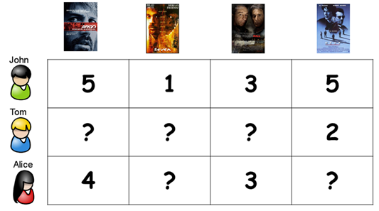
The dictionary meaning of explicit is to state clearly and in detail. Explicit feedback data as the name suggests is an exact number given by a user to a product. Some of the examples of explicit feedback are ratings of movies by users on Netflix, ratings of products by users on Amazon. Explicit feedback takes into consideration the input from the user about how they liked or disliked a product. Explicit feedback data are quantifiable.
Explicit data should be like in the form of ratings.
When was the last time you rated a movie on Netflix? People normally rate a movie or an item on extreme feelings — either they really like the product or when they just hated it. The latter being more prominent. So, chances are your dataset will be largely filled with a lot of positive ratings but very less negative ratings.
Explicit feedback is hard to collect as they require additional input from the users. They need a separate system to capture this type of data. Then you’ve to decide whether you should go with ratings or like/dislike option to collect the feedback. Each having their merits/demerits.
Explicit feedback doesn’t take into consideration the context of when you were watching the movie. Let us understand with an example. You watched a documentary and you really liked it and you rated it well. Now, this doesn’t mean you would like to see a lot many documentaries but with explicit ratings, this becomes difficult to take into consideration. I like to binge watch The Office tv series while having dinner and I would give it a high rating 4.5/5 but that doesn’t mean that I would watch it at any time of the day.
There is another problem with explicit ratings. People rate movies/items differently. Some are lenient with their ratings while others are particular about what ratings they give. You need to take care of bias in ratings from users as well.
Implicit data :
The dictionary meaning of implicit is suggested though not stated clearly. And that’s exactly what implicit feedback data represents. Implicit feedback doesn’t directly reflect the interest of the user but it acts as a proxy for a user’s interest.
Examples of implicit feedback datasets include browsing history, clicks on links, count of the number of times a song is played, the percentage of a webpage you have scrolled — 25%, 50% or 75 % or even the movement of your mouse.
If you just browsed an item that doesn’t necessarily mean that you liked that item but if you have browsed this item multiple times that gives us some confidence that you may be interested in that item. Implicit feedback collects information about the user’s actions.
Implicit feedback data are found in abundance and are easy to collect. They don’t need any extra input from the user. Once you have the permission of the user to collect their data, your dependence on the user is reduced.
Let us talk about some unique characteristics of implicit feedback datasets:
No negative preference measured directly – Unlike explicit feedback where a user gives a poor rating for an item, he/she doesn’t like, we do not have a direct way to measure the interest of a user. Repeated action in favor of the item — for eg. listening to Coldplay’s Fix You gives us confidence that the user likes this song and we could recommend a similar song to the user. However, an absence of listening count for a song doesn’t mean that the user does not like the item — may be the user is not even aware of the existence of the song. So, there is no way to measure negative preference directly.
The numerical value of implicit feedback denotes confidence that the user likes the item – For eg., if I’ve listened to Coldplay more number of times than that to Pink Floyd on Youtube, the system would infer with higher confidence about my likeability for Coldplay.
A lot of noisy data to take care of – You need to do a lot of filtering before you actually can get worthwhile data to be modeled upon. Just because I bought an item doesn’t mean I liked the item — may be I bought it for a friend or maybe I didn’t like the item at all after purchasing the item. To handle such issues, we can calculate confidence associated with the preference of the users for items.
There are two ways to build a recommendation system:-
Content-based Recommendation system :
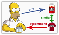
One popular technique of recommendation systems is content-based filtering. Content here refers to the content or attributes of the products you like. So, the idea in content-based filtering is to tag products using certain keywords, understand what the user likes, look up those keywords in the database and recommend different products with the same attributes.
It is based on the idea of recommending the item to user K which is similar to previous item highly rated by K. Basic concept in content based filtering is TF-IDF (Term frequency — inverse document frequency), which is used to determine the importance of document/word/movie etc. Content based filtering shows transparency in recommendation but unlike collaborative filtering it can’t able to work efficiently for large data
Content-based algorithms are given user preferences for items and recommend similar items based on a domain-specific notion of item content. This approach also extends naturally to cases where item metadata is available (e.g., movie stars, book authors, and music genres).
Recommender systems are active information filtering systems that personalize the information coming to a user based on his interests, relevance of the information, etc. Recommender systems are used widely for recommending movies, articles, restaurants, places to visit, items to buy, and more.
Content-based approach requires a good amount of information of items’ own features, rather than using users’ interactions and feedbacks. For example, it can be movie attributes such as genre, year, director, actor etc., or textual content of articles that can extracted by applying Natural Language Processing.
How do Content-based recommender systems work?
A content based recommender works with data that the user provides, either explicitly (rating) or implicitly (clicking on a link). Based on that data, a user profile is generated, which is then used to make suggestions to the user. As the user provides more inputs or takes actions on the recommendations, the engine becomes more and more accurate. The concepts of Term Frequency (TF) and Inverse Document Frequency (IDF) are used in information retrieval and also content based filtering mechanisms (such as a content based recommender). They are used to determine the relative importance of a document / article / news item / movie etc.
Term Frequency (TF) and Inverse Document Frequency (IDF)
The TF*IDF algorithm is used to weigh a keyword in any document and assign the importance to that keyword based on the number of times it appears in the document. Put simply, the higher the TF*IDF score (weight), the rarer and more important the term, and vice versa.
Each word or term has its respective TF and IDF score. The product of the TF and IDF scores of a term is called the TF*IDF weight of that term.
The TF (term frequency) of a word is the number of times it appears in a document. When you know it, you’re able to see if you’re using a term too often or too infrequently.
TF(t) = (Number of times term t appears in a document) / (Total number of terms in the document).
The IDF (inverse document frequency) of a word is the measure of how significant that term is in the whole corpus.
IDF(t) = log_e(Total number of documents / Number of documents with term t in it).
In Python, scikit-learn provides you a pre-built TF-IDF vectorizerthat calculates the TF-IDF score for each document’s description, word-by-word. tf = TfidfVectorizer(analyzer=’word’, ngram_range=(1, 3), min_df=0, stop_words=’english’)
tfidf_matrix = tf.fit_transform(ds[‘description’])
Vector Space Model
In this model, each item is stored as a vector of its attributes (which are also vectors) in an n-dimensional space, and the angles between the vectors are calculated to determine the similarity between the vectors.
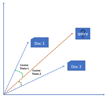
The method of calculating the user’s likes / dislikes / measures is calculated by taking the cosine of the anglebetween the user profile vector (Ui )and the document vector; or in our case, the angle between two document vectors.
The ultimate reason behind using cosine is that the value of cosine will increase as the angle between vectors with decreases, which signifies more similarity. The vectors are length-normalized, after which they become vectors of length 1.
How does Vector Space Model works?
In this model, each item is stored as a vector of its attributes (which are also vectors) in an n-dimensional space and the angles between the vectors are calculated to determine the similarity between the vectors. Next, the user profile vectors are also created based on his actions on previous attributes of items and the similarity between an item and a user is also determined in a similar way.
Calculating Cosine Similarity
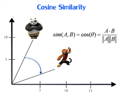
Here we’ve calculated the cosine similarity of each item with every other item in the dataset, and then arranged them according to their similarity with item i, and stored the values in results.
Collaborative Filtering based Recommendation system:
Collaborative methods for recommender systems are methods that are based solely on the past interactions recorded between users and items in order to produce new recommendations. These interactions are stored in the so-called “user-item interactions matrix”.
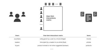
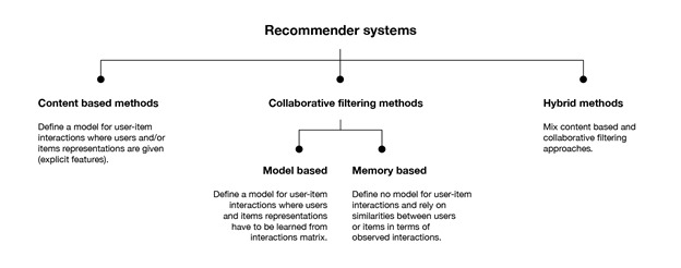
The class of collaborative filtering algorithms is divided into two sub-categories that are generally called memory based and model based approaches.
Memory based approaches directly works with values of recorded interactions, assuming no model, and are essentially based on nearest neighbours search (for example, find the closest users from a user of interest and suggest the most popular items among these neighbours).
Model based approaches assume an underlying “generative” model that explains the user-item interactions and try to discover it in order to make new predictions.
The main advantage of collaborative approaches is that they require no information about users or items and, so, they can be used in many situations. Moreover, the more users interact with items the more new recommendations become accurate: for a fixed set of users and items, new interactions recorded over time bring new information and make the system more and more effective.
However, as it only consider past interactions to make recommendations
we will mainly present three classical collaborative filtering approaches: two memory based methods (user-user and item-item) and one model based approach (matrix factorization).
Memory-based:
User-User:
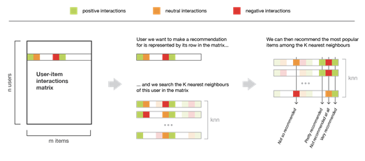
In order to make a new recommendation to a user, user-user method roughly tries to identify users with the most similar “interactions profile” (nearest neighbours) in order to suggest items that are the most popular among these neighbours (and that are “new” to our user). This method is said to be “user-centred” as it represent users based on their interactions with items and evaluate distances between users.
Assume that we want to make a recommendation for a given user. First, every user can be represented by its vector of interactions with the different items (“its line” in the interaction matrix). Then, we can compute some kind of “similarity” between our user of interest and every other users. That similarity measure is such that two users with similar interactions on the same items should be considered as being close. Once similarities to every users have been computed, we can keep the k-nearest-neighbours to our user and then suggest the most popular items among them (only looking at the items that our reference user has not interacted with yet).
Item-Item:
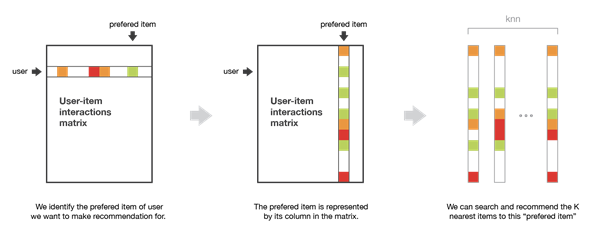
To make a new recommendation to a user, the idea of item-item method is to find items similar to the ones the user already “positively” interacted with. Two items are considered to be similar if most of the users that have interacted with both of them did it in a similar way. This method is said to be “item-centred” as it represent items based on interactions users had with them and evaluate distances between those items
Assume that we want to make a recommendation for a given user. First, we consider the item this user liked the most and represent it (as all the other items) by its vector of interaction with every users (“its column” in the interaction matrix). Then, we can compute similarities between the “best item” and all the other items. Once the similarities have been computed, we can then keep the k-nearest-neighbors to the selected “best item” that are new to our user of interest and recommend these items.
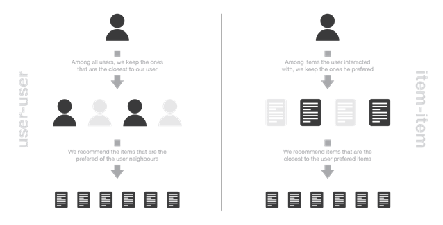
Nearest Neighborhood
The standard method of Collaborative Filtering is known as Nearest Neighborhood algorithm. There are user-based CF and item-based CF. Let’s first look at User-based CF. We have an n × m matrix of ratings, with user uᵢ, i = 1, …n and item pⱼ, j=1, …m. Now we want to predict the rating rᵢⱼ if target user i did not watch/rate an item j. The process is to calculate the similarities between target user i and all other users, select the top X similar users, and take the weighted average of ratings from these X users with similarities as weights.
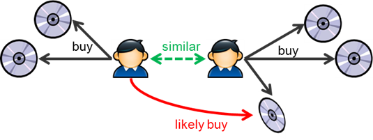
Nearest Neighbor item based-collaborative filtering
Example
Pivot Matrix-
| UserID | 1 | 2 | 3 | 4 |
| Title1 | 4 | NaN | NaN | NaN |
| Title2 | NaN | 4 | NaN | NaN |
| Title3 | NaN | NaN | 5 | NaN |
| Title4 | Nan | 3 | 5 | NaN |
In this table, all the values are Ratings.
Technique Used – Cosine Similarity
Once Our Pivot Matrix is generated I will convert this into an Array Matrix by using csr_matrix
|
1 |
from scipy.sparse import csr_matrix |
Cosine Similarity – sim(A,B)=cos(Theta)=A.B/||A||||B||
In KnearestNeighbor we are going to use the cosine similarity.
We will use KNN which works on Euclidean Distance, In this we will also use Cosine Similarity for to find out the similarity score.
|
1 2 3 |
from scipy.sparse import csr_matrix feature_matrix=csr_matrix(us_canada_user_rating_pivot.values) from sklearn.neighbors import NearestNeighbors |
After fitting that matrix we will use kneighbors for to find out which books/products are Similar. In this By Applying Collaborative filtering using K-NearestNeighbors, we will convert that 2D Matrix into and fill missing values with zeroes others with given ratings, Now we will calculate distances between rating vectors, then we will transform the values(ratings) of matrix dataframe into a scipy sparse for more efficient calculations.
After fitting & applying NearestNeighbors ->
This will find the distances/closeness of instances. It then classifies an instance by finding the Nearest Neighbors and picks the most popular & closer class.
Collaborative Filtering using k-Nearest Neighbors (kNN)
kNN is a machine learning algorithm to find clusters of similar users based on common book ratings, and make predictions using the average rating of top-k nearest neighbors. For example, we first present ratings in a matrix, with the matrix having one row for each item (book) and one column for each user, like so:

We then find the k item that have the most similar user engagement vectors. In this case, Nearest Neighbors of item id 5= [7, 4, 8, …]. Now let’s implement kNN into our book recommender system.
Data
We are using the same book data we used the last time: it consists of three tables: ratings, books info, and users info.
|
1 2 3 4 5 6 7 8 9 |
import pandas as pd import numpy as np from scipy.sparse import csr_matrix import seaborn from sklearn.decomposition import TruncatedSVD from sklearn.neighbors import NearestNeighbors book=pd.read_csv("BX-Books.csv",sep=";",error_bad_lines=False,encoding="latin-1") book.columns=['ISBN','bookTitle','bookAuthor','yearOfPublication','publisher','imageUrlS','imageUrlM','imageUrlL'] |
|
1 2 3 |
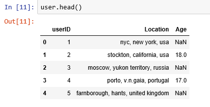
user=pd.read_csv("BX-Users.csv",sep=";",error_bad_lines=False,encoding="latin-1") user.columns=['userID','Location','Age'] |
|
1 2 |
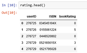
rating=pd.read_csv("BX-Book-Ratings.csv",sep=";",error_bad_lines=False,encoding="latin-1") rating.columns=['userID','ISBN','bookRating'] |
Rating info
|
1 |
rating.head() |
User info
|
1 |
user.head() |
Book info
|
1 |
book.head() |
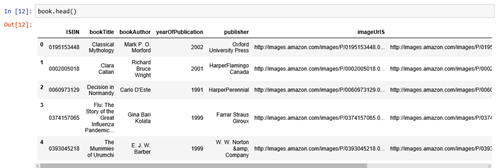
To ensure statistical significance, we will be only looking at the popular books
In order to find out which books are popular, we need to combine book data with rating data.
|
1 2 3 4 |
combine_book_rating=pd.merge(book,rating,on="ISBN") columns=['yearOfPublication','publisher','bookAuthor','imageUrlS','imageUrlM','imageUrlL'] combine_book_rating=combine_book_rating.drop(columns,axis=1) combine_book_rating.head() |
We then group by book titles and create a new column for total rating count.
|
1 2 3 4 5 6 7 8 9 10 11 12 |
combine_book_rating=combine_book_rating.dropna(axis=0,subset=['bookTitle']) combine_book_rating.head() combine_book_rating[['bookTitle','bookRating']].info() combine_book_rating.describe() book_ratingCount=(combine_book_rating. groupby(by=['bookTitle'])['bookRating']. count(). reset_index(). rename(columns={'bookRating':'totalRatingCount'}) [['bookTitle','totalRatingCount']] ) book_ratingCount.head() |
we now combine the rating data with the total rating count data, this gives us exactly what we need to filter out the lesser known books.
|
1 2 3 4 5 |
rating_with_totalRatingCount=combine_book_rating.merge(book_ratingCount,left_on='bookTitle',right_on='bookTitle',how="inner") rating_with_totalRatingCount.head() rating_with_totalRatingCount.info() rating_with_totalRatingCount.describe() rating_with_totalRatingCount['totalRatingCount'].count() |
In this we have done filtering those who have popularity means totalRatingCount whose greater than 50
|
1 2 3 4 |
popularity_threshold=50 #rating_popular_book=rating_with_totalRatingCount.query('totalRatingCount>=@popularity_threshold') rating_popular_book=rating_with_totalRatingCount[rating_with_totalRatingCount['totalRatingCount']>popularity_threshold] rating_popular_book.head() |
Filter to users in US and Canada only
In order to improve computing speed, and not run into the “MemoryError” issue, I will limit our user data to those in the US and Canada.
|
1 2 3 4 5 6 7 8 |
#I am filtering the users data to only US and Canada only combined=rating_popular_book.merge(user,left_on='userID',right_on='userID',how="inner") combined.head() us_canada_user_rating = combined[combined['Location'].str.contains("usa|canada")] us_canada_user_rating.head() us_canada_user_rating=us_canada_user_rating.drop(['Age'],axis=1) us_canada_user_rating.head() us_canada_user_rating=us_canada_user_rating.drop_duplicates(['userID','bookTitle']) |
Implementing kNN
We convert our table to a 2D matrix, and fill the missing values with zeros (since we will calculate distances between rating vectors). We then transform the values(ratings) of the matrix dataframe into a scipy sparse matrix for more efficient calculations.
Finding the Nearest Neighbors
We use unsupervised algorithms with sklearn.neighbors. The algorithm we use to compute the nearest neighbors is “brute”, and we specify “metric=cosine” so that the algorithm will calculate the cosine similarity between rating vectors. Finally, we fit the model.
|
1 2 3 |
us_canada_user_rating_pivot=us_canada_user_rating.pivot(index="bookTitle",columns="userID",values="bookRating").fillna(0) us_canada_user_rating_pivot us_canada_user_rating_pivot.shape |
|
1 2 3 |
us_canada_user_rating_matrix=csr_matrix(us_canada_user_rating_pivot.values) us_canada_user_rating_matrix us_canada_user_rating_pivot |
Test our Model And Make Recommendations:
In this step, the kNN algorithm measures distance to determine the “closeness” of instances. It then classifies an instance by finding its nearest neighbors, and picks the most popular class among the neighbors.
|
1 2 3 |
from sklearn.neighbors import NearestNeighbors model_knn=NearestNeighbors(metric="cosine",algorithm="brute") model_knn.fit(us_canada_user_rating_matrix) |
|
1 2 3 4 5 6 7 8 9 10 11 12 13 14 15 |
#query_index=np.random.choice(us_canada_user_rating_pivot.shape[0]) query_index=2378 #print(us_canada_user_rating_pivot.iloc[query_index,:]) distances,indices=model_knn.kneighbors(us_canada_user_rating_pivot.iloc[query_index,:].values.reshape(1,-1),n_neighbors=6) print("Distances -->",distances," Indices -->",indices) print(distances.flatten()) print(len(distances.flatten())) for i in range(0,len(distances.flatten())): if i==0: print("Recommendation for {0}:\n".format(us_canada_user_rating_pivot.index[query_index])) else: print("{0}: {1}, with distance of {2}:".format(i,us_canada_user_rating_pivot.index[indices.flatten()[i]],distances.flatten()[i])) |
This is our Books Recommendation Model, In this KNearestNeighbors I have used Explicit Ratings to build this model And by using this same technique we are able to build any recommendation system.
Related content
Auriga: Leveling Up for Enterprise Growth!
Auriga’s journey began in 2010 crafting products for India’s
