Dimensionality Reduction : PCA, tSNE, UMAP

Why dimensionality reduction ?

Dimensionality reduction is a technique used in machine learning and data analysis to reduce the number of input variables or features in a dataset while retaining the most important information. The process involves transforming high-dimensional data into a lower-dimensional space, where each dimension represents a combination of the original features.

The main goal of dimensionality reduction is to simplify the dataset by eliminating redundant or irrelevant features, which can lead to several benefits:

1. Computational efficiency: High-dimensional data can be computationally expensive to process and analyze. By reducing the dimensionality, the computational complexity can be significantly reduced, making the algorithms more efficient.
2. Noise reduction: Dimensionality reduction can help in filtering out noisy or irrelevant features, which can negatively impact the performance of machine learning models. By focusing on the most informative dimensions, the models can achieve better generalization and predictive accuracy.
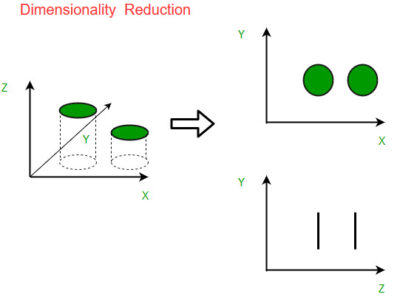
3. Visualization: Visualizing high-dimensional data is challenging, as humans can only perceive up to three dimensions directly. Dimensionality reduction techniques enable the representation of data in two or three dimensions, allowing for easier visualization and interpretation.
4. Feature engineering: Dimensionality reduction can assist in feature engineering by creating new, derived features that capture the most relevant information in the original dataset. These derived features can then be used as inputs for subsequent machine learning models.

There are two main approaches to dimensionality reduction:

1. Feature selection: This approach involves selecting a subset of the original features based on certain criteria such as statistical tests, correlation analysis, or domain knowledge. The selected features are retained, while the rest are discarded.
2. Feature extraction: In this approach, new features are created by combining or transforming the original features. The goal is to find a lower-dimensional representation that preserves the most important information from the original data. Techniques like Principal Component Analysis (PCA), Linear Discriminant Analysis (LDA), and t-distributed Stochastic Neighbor Embedding (t-SNE) are commonly used for feature extraction.

Principal Component Analysis (PCA): 

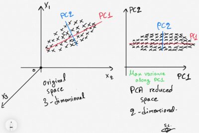
PCA, or Principal Component Analysis, is a widely used dimensionality reduction technique. The basic idea behind PCA is to identify patterns in the relationships between variables, and to represent these patterns in terms of a smaller number of variables, called principal components. The procedure for PCA typically involves the following steps :

1. Standardization: If the input variables have different scales, it is common to standardize them to have zero mean and unit variance. This step ensures that each variable contributes equally to the analysis.
2. Covariance matrix calculation: The next step is to compute the covariance matrix of the standardized data. The covariance matrix describes the relationships between pairs of variables and provides information about their joint variability.
3. Eigenvalue decomposition: The covariance matrix is then decomposed into its eigenvectors and eigenvalues. The eigenvectors represent the directions or principal components of the data, and the eigenvalues indicate the amount of variance explained by each principal component. The eigenvectors are sorted in descending order based on their corresponding eigenvalues.
4. Selection of principal components: The next step involves selecting a subset of the principal components to retain. This decision can be based on the cumulative explained variance, where the eigenvalues are normalized and summed. A common approach is to choose the top-k principal components that explain a significant amount of the total variance (e.g., 95% or 99%).
5. Projection: The selected principal components are used to create a new feature subspace. The original data are projected onto this subspace to obtain the transformed dataset with reduced dimensionality. This projection is done by multiplying the standardized data by the matrix of selected eigenvectors.

t-Distributed Stochastic Neighbor Embedding (t-SNE) :  

The basic idea behind t-SNE is to convert similarities between data points in the high-dimensional space into probabilities, and then map these probabilities to a lower-dimensional space in a way that preserves the relationships between the data points as much as possible. The procedure for t-SNE involves the following steps :

1. Compute pairwise similarities: First, pairwise similarities between data points in the high-dimensional space are computed. These similarities are typically calculated using a Gaussian kernel that measures the similarity based on the Euclidean distance between data points.
2. Construct probability distributions: From the pairwise similarities, probability distributions are constructed for each data point. The distributions represent the similarities between a data point and all other points in the high-dimensional space. The similarities are converted into probabilities using the softmax function.
3. Initialize embedding: An initial embedding of the data points in the low-dimensional space is randomly generated. Each data point is assigned a position in the low-dimensional space.
4. Compute similarity in low-dimensional space: Similar to the high-dimensional space, pairwise similarities between data points are computed in the low-dimensional space. However, in the low-dimensional space, a different distribution is used, called the Student’s t-distribution, to model the pairwise similarities.
5. Optimize embedding: The goal of t-SNE is to minimize the divergence between the pairwise similarities in the high-dimensional space and the pairwise similarities in the low-dimensional space. This is achieved through an iterative optimization process. The positions of the data points in the low-dimensional space are adjusted iteratively to minimize the difference between the high-dimensional and low-dimensional pairwise similarities. The optimization is typically performed using gradient descent.
6. Convergence: The optimization process continues until a stopping criterion is met. This criterion can be a maximum number of iterations, a desired level of convergence, or a threshold for the change in the embedding positions.
7. Visualization: Once the optimization is complete, the final low-dimensional embedding can be visualized. Data points are plotted in the low-dimensional space, where their positions are determined by the optimized embedding. The visualization aims to represent the similarities and relationships between data points in a way that preserves the local and global structure of the high-dimensional data.

 

Uniform Manifold Approximation and Projection (UMAP) : 

The basic idea behind UMAP is to construct a low-dimensional representation of the data that preserves the global and local structure of the high-dimensional space. UMAP uses a graph-based approach to build a topological representation of the data, which is then embedded in a low-dimensional space using stochastic gradient descent. The procedure for UMAP involves the following steps:

1. Compute the pairwise distances: The first step is to calculate the pairwise distances between data points in the high-dimensional space. The choice of distance metric depends on the nature of the data and the problem at hand. Common distance metrics include Euclidean distance, cosine distance, or correlation distance.
2. Construct a fuzzy simplicial set: Based on the pairwise distances, a fuzzy simplicial set is constructed. A fuzzy simplicial set represents the local neighborhood structure of the data points. It captures the notion of “nearness” or “similarity” between data points, taking into account the density and connectivity of the data.
3. Optimize the low-dimensional embedding: The goal of UMAP is to find a low-dimensional representation that preserves the neighborhood relationships captured by the fuzzy simplicial set. This is done through an optimization process. Initially, a random low-dimensional embedding is generated. Then, UMAP uses stochastic gradient descent to minimize the discrepancy between the pairwise similarities in the high-dimensional space and the low-dimensional space.
4. Construct a graph and perform graph layout: UMAP constructs a graph representation based on the low-dimensional embedding. This graph captures the global structure of the data. Graph layout algorithms, such as force-directed layout or spectral layout, are applied to position the data points in the low-dimensional space, taking into account the graph structure.
5. Refine the embedding: UMAP performs a refinement step to improve the embedding further. This step involves adjusting the positions of the data points based on the graph structure and the connectivity of the data.
6. Convergence: The optimization and refinement steps are iterated until convergence is achieved. Convergence can be determined based on a specified number of iterations or a stopping criterion, such as a threshold for the change in the embedding positions.
7. Visualization and analysis: Once the optimization is complete, the final low-dimensional embedding can be visualized and analyzed. The low-dimensional representation aims to preserve the neighborhood relationships and the global structure of the high-dimensional data. It can be used for visualization, clustering, or further analysis tasks.

Comparison among PCA, t-SNE and UMAP : 

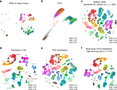
1. Linear vs. Nonlinear: PCA is a linear dimensionality reduction technique that focuses on finding orthogonal axes that explain the maximum variance in the data. It is effective for capturing global patterns and reducing the dimensionality of data. In contrast, t-SNE and UMAP are nonlinear techniques that aim to preserve both local and global structures in the data, making them more suitable for visualizing and exploring complex relationships.
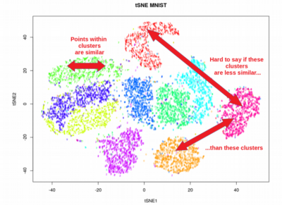
2. Preservation of global vs. local structure: PCA primarily focuses on preserving the global structure of the data, meaning it aims to capture the overall variance and trends in the dataset. It may not preserve the fine-grained local structure or clustering patterns in the data. On the other hand, t-SNE and UMAP excel at preserving the local structure, emphasizing the relationships between nearby data points. They can reveal clusters, patterns, and nonlinear relationships that may be hidden in high-dimensional space.
3. Computation time and scalability: PCA is computationally efficient and can handle large datasets. It is a linear algebra-based technique that can be efficiently computed using matrix operations. t-SNE and UMAP, on the other hand, are more computationally intensive, especially for large datasets. They involve optimization procedures and graph-based computations, which can be time-consuming. UMAP is designed to be more scalable than t-SNE and can handle large-scale datasets more efficiently.
4. Interpretability: PCA provides interpretable results as the principal components represent linear combinations of the original features. Each principal component captures a certain amount of variance in the data, and their contributions can be analyzed. In contrast, t-SNE and UMAP produce transformed embeddings in a lower-dimensional space that are not directly interpretable in terms of the original features. They are primarily used for visualization and exploration purposes.
5. Suitability for different tasks: PCA is commonly used for dimensionality reduction, feature selection, and noise reduction. It is also used as a preprocessing step for various machine learning algorithms. t-SNE and UMAP are often employed for data visualization and exploration. They help reveal complex structures, clusters, and relationships in the data, making them valuable for tasks such as exploratory data analysis, pattern recognition, and anomaly detection.
6. Parameter tuning: PCA does not have many tunable parameters. The number of principal components to retain is a key decision, which can be based on variance explained or domain knowledge. t-SNE and UMAP have more parameters to adjust. For example, in t-SNE, the perplexity, learning rate, and number of iterations influence the results. UMAP has parameters such as n_neighbors, min_dist, and metric that affect the embedding quality.

Tensorflow Embedding Projector :

The TensorFlow Embedding Projector is a web-based visualization tool provided by TensorFlow, an open-source machine learning framework developed by Google. It is designed specifically for visualizing high-dimensional embeddings, such as word embeddings or learned representations of data, in a lower-dimensional space.

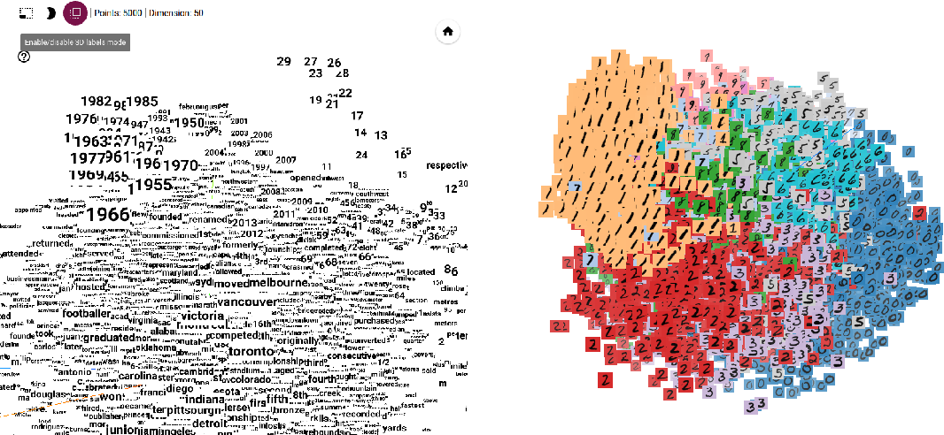
The TensorFlow Embedding Projector allows users to interactively explore and analyze embeddings, providing valuable insights into the relationships, clusters, and patterns within the data. It offers several features and functionalities, including:

1. 3D Scatter Plot: The Embedding Projector provides a 3D scatter plot visualization, allowing users to navigate and inspect the embeddings from different angles. Data points are represented as markers, and users can zoom, rotate, and pan the plot to explore the spatial relationships between the embeddings.
2. Labels and Metadata: Users can assign labels to the data points, providing additional information about each embedding. Labels can be used to identify specific categories, classes, or entities associated with the data. Furthermore, metadata, such as additional attributes or properties of the embeddings, can be attached to each data point for further analysis.
3. Coloring and Filtering: The Embedding Projector enables users to color the data points based on specific attributes or labels, making it easier to identify clusters or visualize patterns. Additionally, users can apply filters to focus on specific subsets of the data, highlighting particular regions or groups of embeddings.
4. Similarity Search: The Embedding Projector includes a similarity search functionality that allows users to find nearest neighbors of a selected data point based on similarity measures. This feature helps identify embeddings with similar characteristics or relationships, aiding in the exploration and analysis of the data.
5. Import and Export: The Embedding Projector supports the import and export of embeddings in various formats, including TensorFlow checkpoints, word2vec formats, and TSV (Tab-Separated Values) files. This flexibility enables users to work with embeddings generated from different models or sources.

hands on