Understanding Yolo (You Look Only Once)

Firstly, We need to understand what is Yolo used for? A groundbreaking algorithm that is used to detects objects in real-time.

So, let’s understand  what is Object Detection?

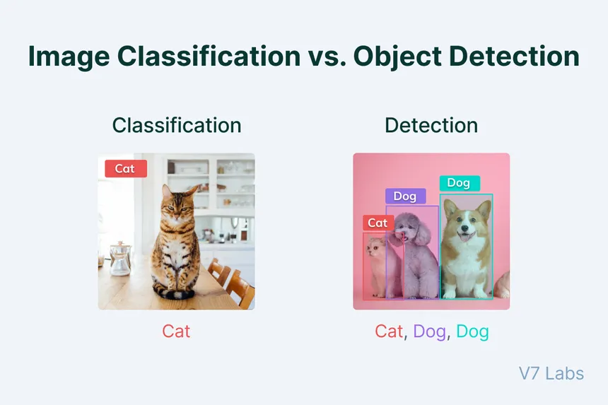
Object Detection –

Object detection, a fundamental task in computer vision, is designed to recognize and locate multiple objects within digital images or videos. This process answers two key questions: “What is the object?” and “Where is it   located?” It involves identifying the types of objects present and precisely determining their positions through bounding boxes or similar markers. Object detection is crucial in applications ranging from autonomous vehicles, where it identifies obstacles and road signs, to security systems, which detect unusual activities or individuals. It combines aspects of image classification and localization to provide a comprehensive understanding of visual scenes.

 

Let’s Understand Yolo –

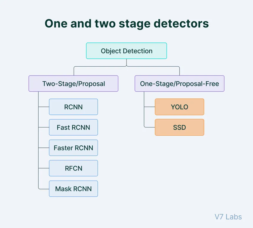
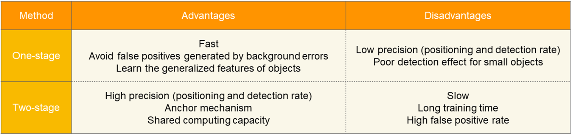
YOLO, an acronym for “You Only Look Once,” is a highly influential algorithm in the field of computer vision, particularly for real-time object detection. This algorithm revolutionizes the way objects are identified and localized in images and videos. Unlike traditional methods that treat object detection as a two-step process (first identifying the object, then localizing it), YOLO integrates these steps into a single, unified process. It processes the entire image at once, predicting what objects are in the image and where they are located. This holistic approach allows for rapid and efficient detection, making YOLO exceptionally well-suited for real-time applications and it is known as One Stage Detection.

 

 

YOLO employs a deep neural network, which looks at the entire image in a single evaluation, thus the name “You Only Look Once.” This method contrasts with prior techniques that would scan over parts of the image multiple times to detect objects.

 

 

The real-time processing capability of YOLO has made it a popular choice in various applications where speed is crucial, such as in autonomous vehicles, surveillance systems, and interactive systems that require immediate, accurate object detection. The successive versions of YOLO have focused on improving accuracy, speed, and the ability to generalize across different types of images, making it a versatile and powerful tool in the evolving field of computer vision.

Working Of Yolo –

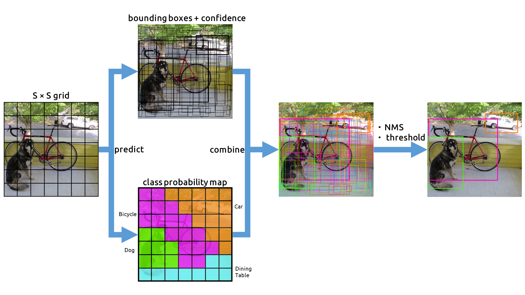
YOLO (You Only Look Once) works by dividing an image into a grid, with each cell in the grid responsible for detecting objects within its boundaries. Every grid cell predicts multiple bounding boxes, each with its own confidence score reflecting the likelihood of an object’s presence. Alongside, it predicts class probabilities indicating the type of object each bounding box may contain. The algorithm combines these predictions to determine the most probable objects and their locations in the image. This process allows YOLO to detect and classify multiple objects simultaneously, contributing to its speed and efficiency in real-time applications.

• Grid Division : YOLO starts by dividing the image into a fixed number of grids, each responsible for detecting objects within its area.
• Bounding Box Prediction : Each grid cell predicts multiple bounding boxes. Each box includes:
• • Coordinates : The center, width, and height of the box.
• • Confidence Score : Reflects the likelihood of an object being present in the box.
• Class Prediction : Alongside bounding boxes, each grid cell predicts the probability of various object classes.
• Combining Predictions : YOLO aggregates the bounding box and class predictions to determine the most probable objects and their locations.
• Filtering Boxes : Using techniques like Non-Maximum Suppression, YOLO filters out overlapping boxes to retain the most accurate predictions.
• Speed and Efficiency : By processing the entire image in a single pass, YOLO achieves remarkable speed, making it suitable for real-time detection tasks.
• End-to-End Learning : The entire process, from grid prediction to class and bounding box determination, is learned end-to-end through a neural network, optimizing accuracy and efficiency.

 

 

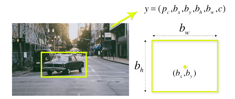
Bounding Box –

A bounding box in object detection is an imaginary rectangle that defines the location of an object in an image. It includes :

Class : Identifies the type of object within the box (e.g., car, truck, person)

Center Coordinates (xc, yc) : The x and y coordinates of the bounding box’s center

Width : The horizontal dimension of the bounding box

Height : The vertical dimension of the bounding box

Confidence : A probability score indicating the likelihood of the object’s presence in the box (e.g., 0.9 confidence implies a 90% certainty that the object is there).

 

 

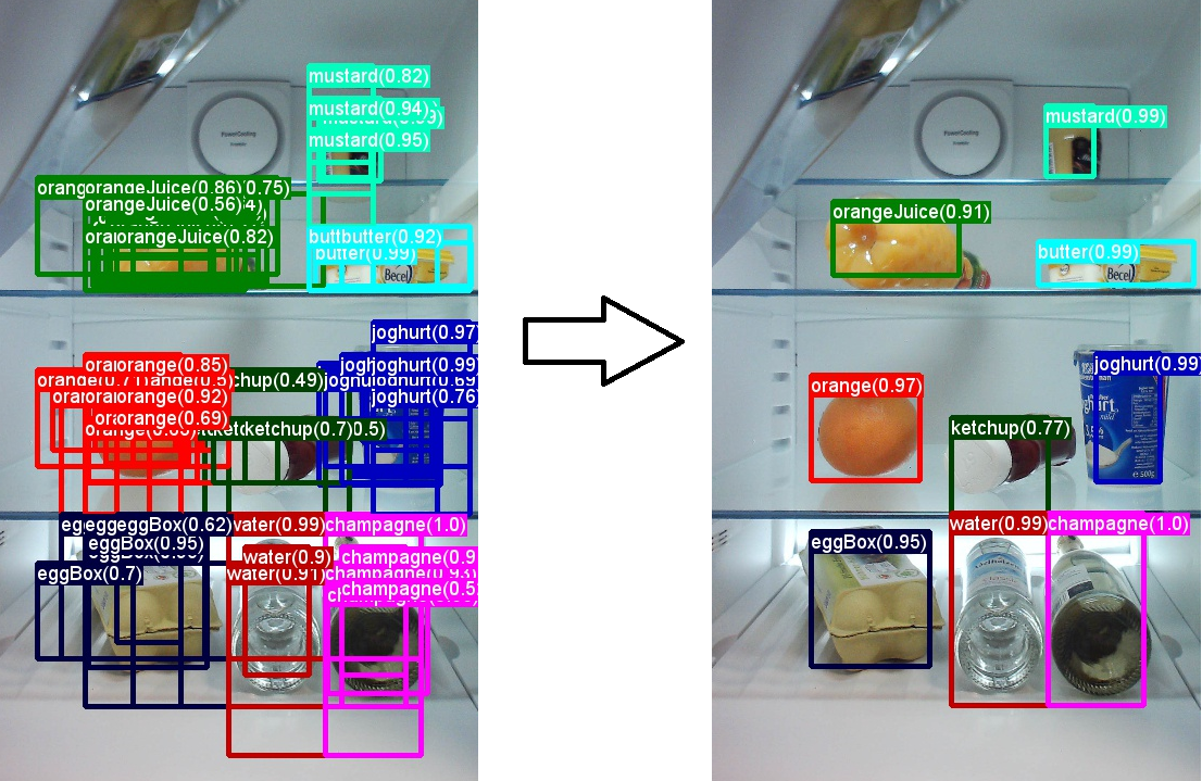
Non Maximal Suppression –

Non-Maximal Suppression (NMS) is a technique in object detection algorithms used to resolve the issue of multiple bounding boxes being detected for the same object. It works by first selecting the bounding box with the highest confidence score, then suppressing all other overlapping boxes with lower scores. This is achieved by comparing the overlap of bounding boxes using metrics like Intersection over Union (IoU). By retaining only the most accurate bounding box for each object and removing redundancies, NMS ensures a cleaner, more precise output in object detection tasks.

Prioritizing High Scores : NMS starts by focusing on bounding boxes with higher confidence scores.

Comparing Overlaps : It compares these boxes to check for overlaps using metrics like Intersection over Union (IoU).

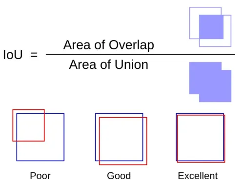
Intersection over Union (IoU) is a crucial metric in object detection:

IOU measures the accuracy of an object detector by calculating the overlap between the predicted bounding box and the ground truth (actual) box.

• Overlap Calculation : It divides the area of overlap between the two boxes by the area of their union.
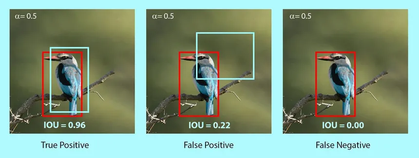
• Accuracy Indicator : A higher IoU value indicates a greater match between the predicted and actual boxes, suggesting more accurate object detection.
• Thresholding : Often, a threshold (e.g., 0.5 IoU) is set to determine whether a prediction is considered accurate.

 

 

 

 

Suppressing Lower Scores : Boxes with significant overlap and lower scores are suppressed, leaving only the box with the highest score in each overlapping group.

Result : The outcome is a cleaner, more accurate set of bounding boxes, ensuring that each detected object is represented only once.

This process is key to eliminating redundant and less accurate predictions.

 

 

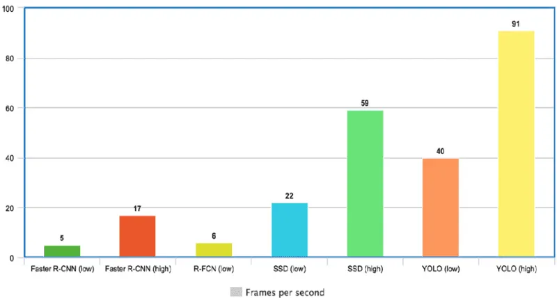
Comparison of Yolo to other Models

Faster R-CNN : Performs at 5 FPS (low quality) and 17 FPS (high quality).

R-FCN : Delivers at 6 FPS, indicating moderate performance.

SSD : Processes at two levels, 22 FPS (low quality) and 59 FPS (high quality), showing good speed.

YOLO : Offers the highest FPS rates, with 40 FPS (low quality) and a significant leap to 91 FPS (high quality), showcasing its superiority in speed.

 

 

Evolution of YOLO – From YOLO to YOLOv8

YOLO or YOLOv1, the starting point

• This first version of YOLO was a game changer for object detection, because of its ability to quickly and efficiently recognize objects.
• It struggles to detect smaller images within a group of images, such as a group of persons in a stadium. This is because each grid in YOLO architecture is designed for single object detection.

YOLOv2 or YOLO9000

• YOLOv2 was created in 2016 with the idea of making the YOLO model better, faster and stronger using Darknet-19 as backbone.
• Batch normalization
• Higher input resolution
• Convolution layers using anchor boxes

YOLOv3 — An incremental improvement

• The change mainly includes a new network architecture: Darknet-53.
• Better bounding box prediction
• More accurate class predictions
• Convolution layers using anchor boxes

YOLOv4 — Optimal Speed and Accuracy of Object Detection

• YOLOv4 is distinguished by its CSPDarknet-53 backbone, which balances speed and accuracy for object detection.
• It outperforms previous YOLO versions and other detectors by achieving higher FPS without compromising on precision, making it ideal for real-time applications that require both quick and reliable object identification.
• Ideal for systems requiring fast, precise object detection.

YOLOv5

• YOLOv5, compared to other versions, does not have a published research paper, and it is the first version of YOLO to be implemented in Pytorch, rather than Darknet.
• The release includes five different model sizes: YOLOv5s (smallest), YOLOv5m, YOLOv5l, and YOLOv5x (largest).

 

YOLOv6 and Yolov7 — A Object Detection Framework for Industrial Applications

• Dedicated to industrial applications with hardware-friendly efficient design and high performance
• Hardware-friendly backbone
• More effective training strategy
• Overall, the improvements in YOLOv6 make it a more accurate, efficient, and deployable object detection model than YOLOv5.

 

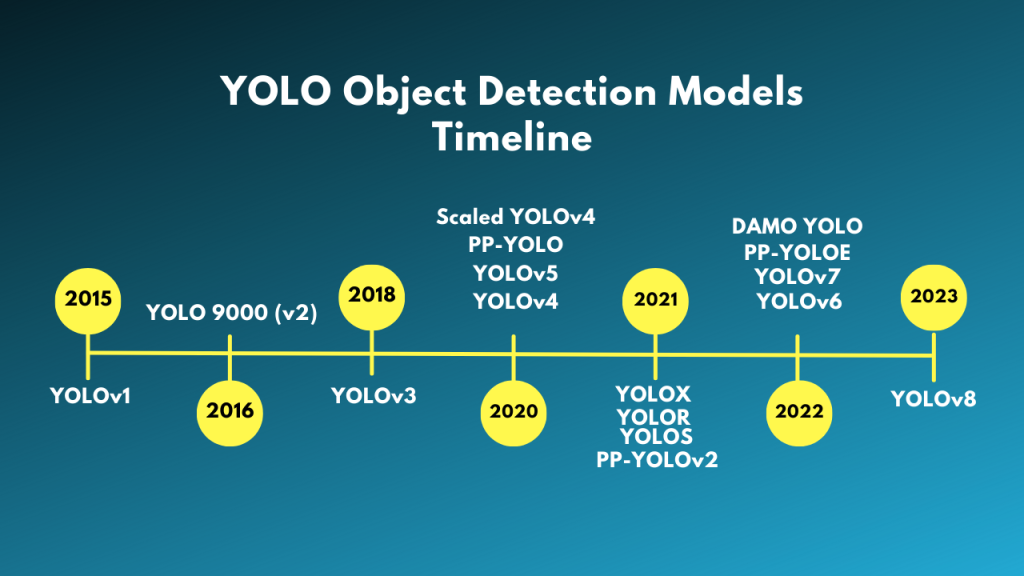
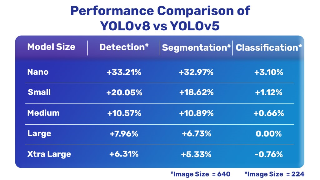
YOLOv8

Ultralytics have released a completely new repository for YOLO Models. It is built as a unified framework for training Object Detection, Instance Segmentation, and Image Classification models.

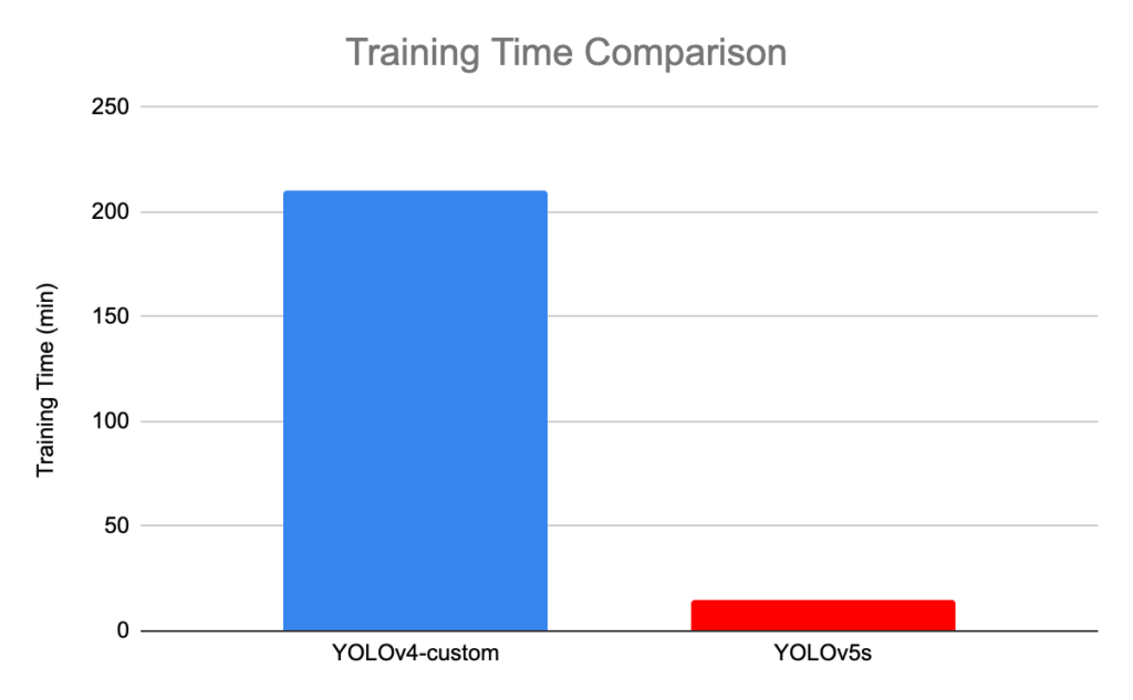
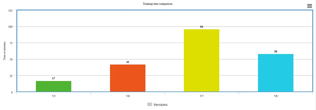
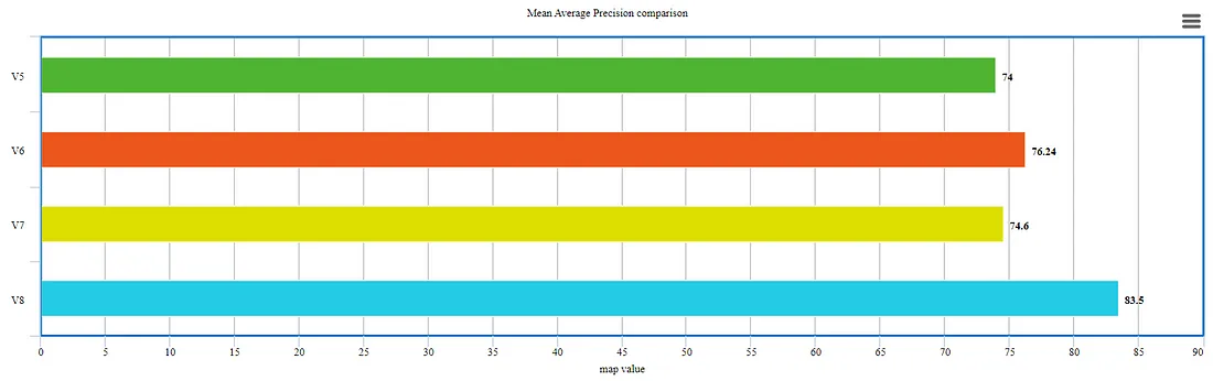
A big concern if we consider the exponential growth from v5 to v7 but v8 is taking almost 60% time to train while producing outcomes with higher mean average precision. Here, the issue of prolonged training is somewhat addressed.

Maximum map value at the expense of reduced time for training. Anchor-free detections are faster and more accurate than the previous version.

 

 

 

 

Practical Implementation

To add a custom dataset configuration for your Yolov8 Model to train test and predict, follow these steps:

1. Create a Dataset Directory : Organize your dataset into a main directory, often named after the dataset version, like ‘dataset_v8’.
2. Subdirectories for Data Splits : Inside the main directory, create three subdirectories: ‘train’, ‘test’, and ‘valid’, each containing images corresponding to training, testing, and validation sets.
3. Configuration File : Draft a ‘yml’ file, specifying the paths to each data split relative to the main dataset directory.
4. Classes and Names : Define the number of classes ‘nc’ in your dataset and list the class names under ‘names’.

 

Folder Structure :

dataset_v8

├── train

│   └── images

├── test

│   └── images

├── valid

│   └── images

└── custom_data.yml

custom_data.yml

Using CLI ( Command Line Interface ) –

For Training :

For Validation :

For Predicting :

Using Python Script –

For Training :

For Validation :

For Predicting :